Chapter 9 File Organization
9.1 Organizing
Writing a research project is more than economic theory, models, and analysis; it also relies on being organized. Most of us have never thought about how to organize multi-year projects because we’ve never had to do them. In this chapter, we will be discussing two topics on the organization side of a research project: file organization and reproducible research papers. This will be less about data cleaning and more about staying organized with R.
File organization is something we all need but are rarely taught. This section closely follows Princeton’s Empirical Study of Conflict (ESOC) research production guide produced by Jacob N. Shapiro. It is highly recommended you read through the production guide.9 The guide goes through file organization as well as best coding practices. Before continuing, it needs to be noted there is no one best way to organize files. At the end of the day, it is what works best FOR YOU! This portion of the book lays out one example of file organization. It is recommended you tweak the ideas discussed in this portion of the Guided Exercise to meet your needs. Remember, file organization is meant to make your life easier.
Before we begin, create a new R Project and name it whatever you want, wherever you want. After creating an R Project, it is time to fill it with all your work. Your base Rproject directory should have every file in a folder except .RData, .Rhistory, lab_diary.txt, the Rproject, project_idea.txt and git_ignore if you’re syncing with Github. Below is an example R Project titled payments_hate_speech:
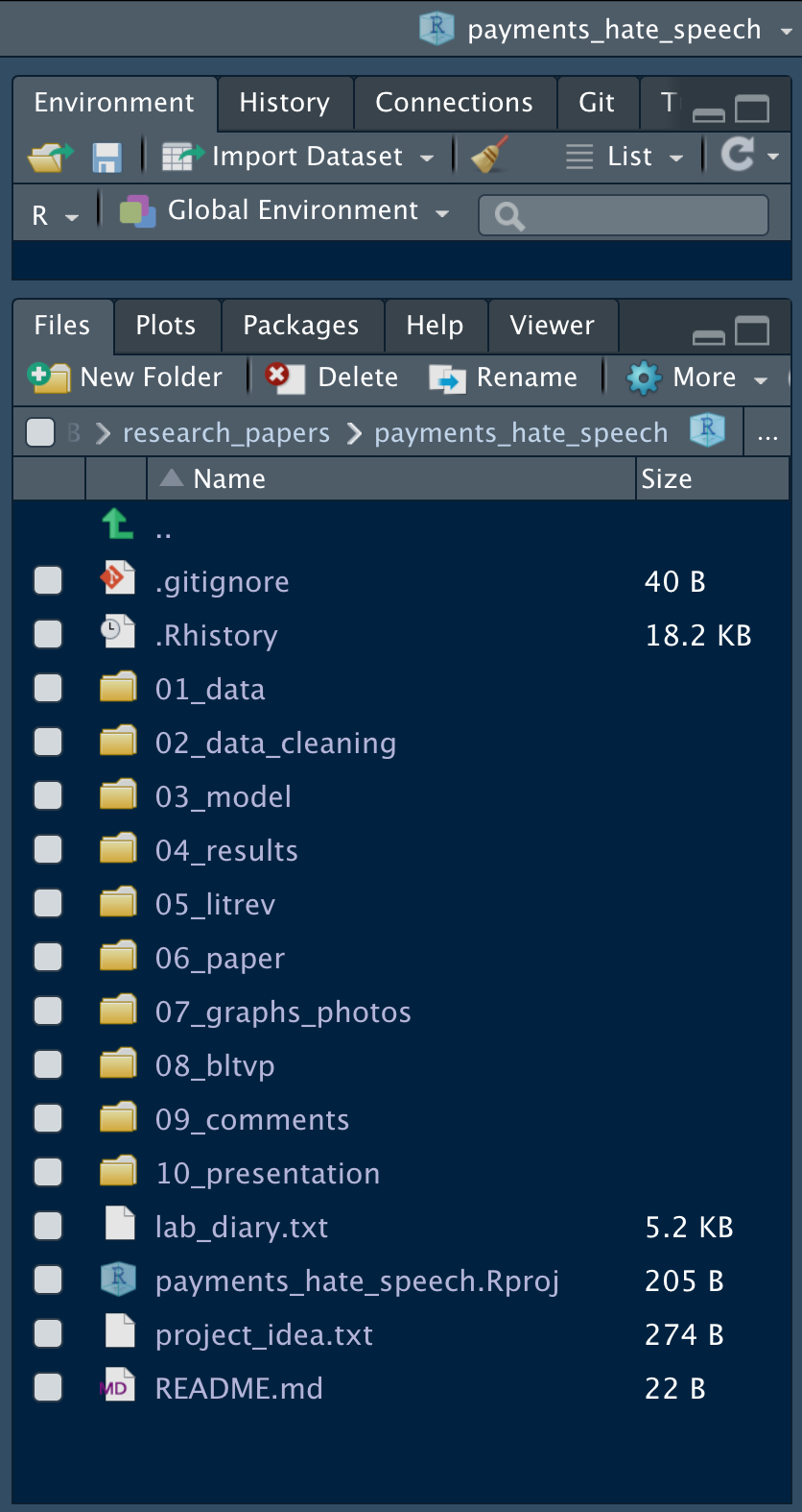
Figure 9.1: Project Layout
Note that all folders are numbers and each number is two digits. The leading zeros are to ensure that the documents are in the correct order (e.g., 01, 02, 03).
Each folder will have a specific purpose with an accompanying README.txt file. The README.txt file should provide a 1-2 sentence description of what the file is/does. If it is raw data, it should say where the data was from. If it is an R script that creates your main data, say that along with what the inputs and outputs are. If it is an R script that makes Table X for your paper, say it does that along with what it inputs/other files it depends on. Write as if you are writing for someone who has never heard of your project nor ever looked at your data. This person may very well be a reviewer. It will also be you a year after you start your project! Figure \(\ref{readme}\) provides an example of a README.txt for the folder 03_model. Each file in the folder has a 1 sentence description, a list of the inputs to the file, and what the file outputs. Notice the local file-paths are included in the inputs and outputs so someone can follow the files. Keeping README.txt files are tedious but incredibility important. If done thoroughly, the data replication needed when submitting papers is already complete. You just send the R Project.
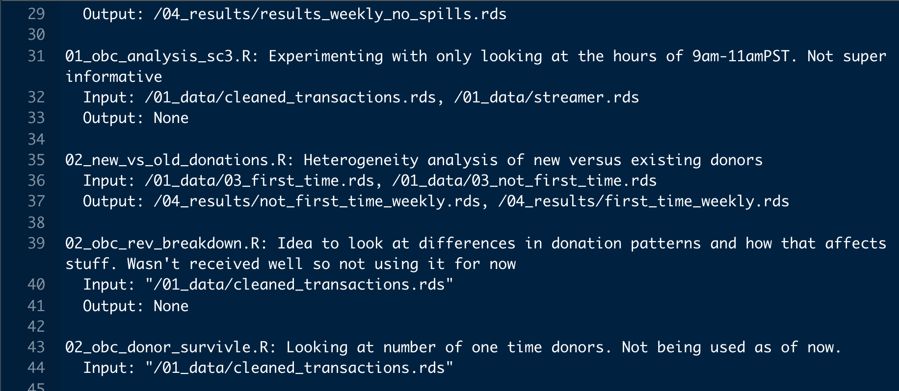
Figure 9.2: README.txt Example for 03_model
The lab_diary.txt is a common tool used in other fields. It’s a place to record what you tried during the day. These notes often come in handy as they cut down the time you spend re-estimating the same regression because you forgot what you did it a week ago. Here is an example of a lab diary.
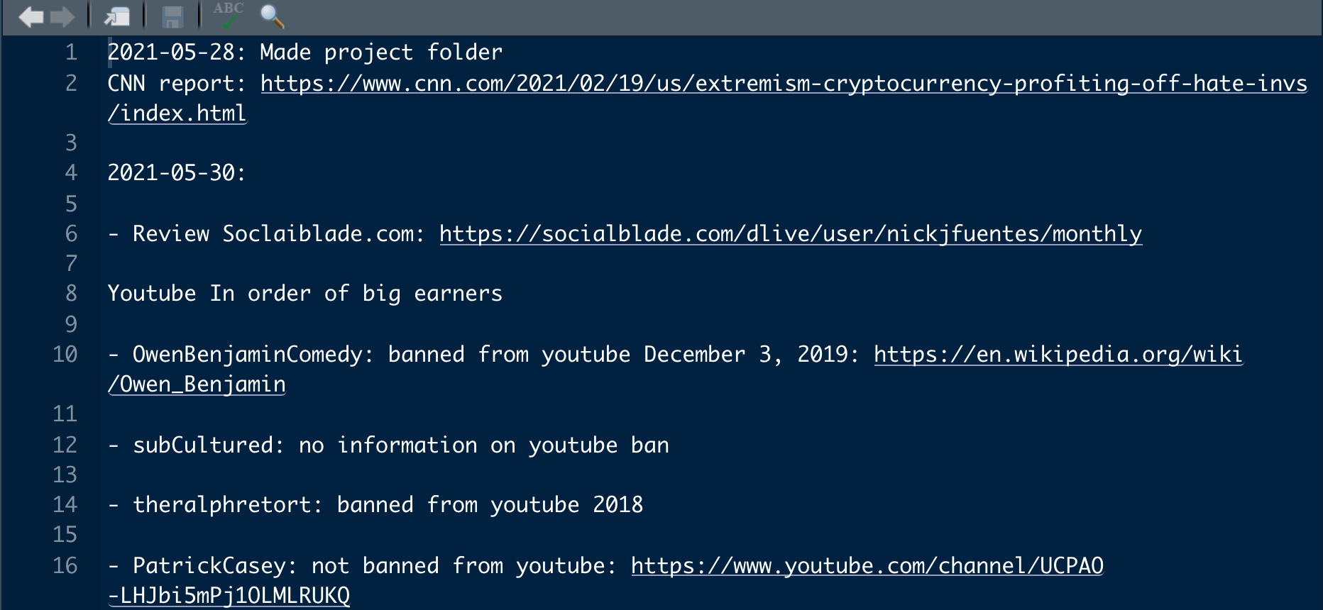
Figure 9.3: Lab Diary
When progressing through your research career, it’s important to figure out an organization style that works best for you. After you find it, create a general template of it. Then, whenever you have a new idea, you can just copy the template and your project is already set up. No more wasting time making folders and thinking about how you want to organize your project. Figure \(\ref{template}\) shows one approach; this approach has one general folder housing all projects, then a template for the project organization. Whenever a new idea comes to mind, the template folder is copied for quick setup.
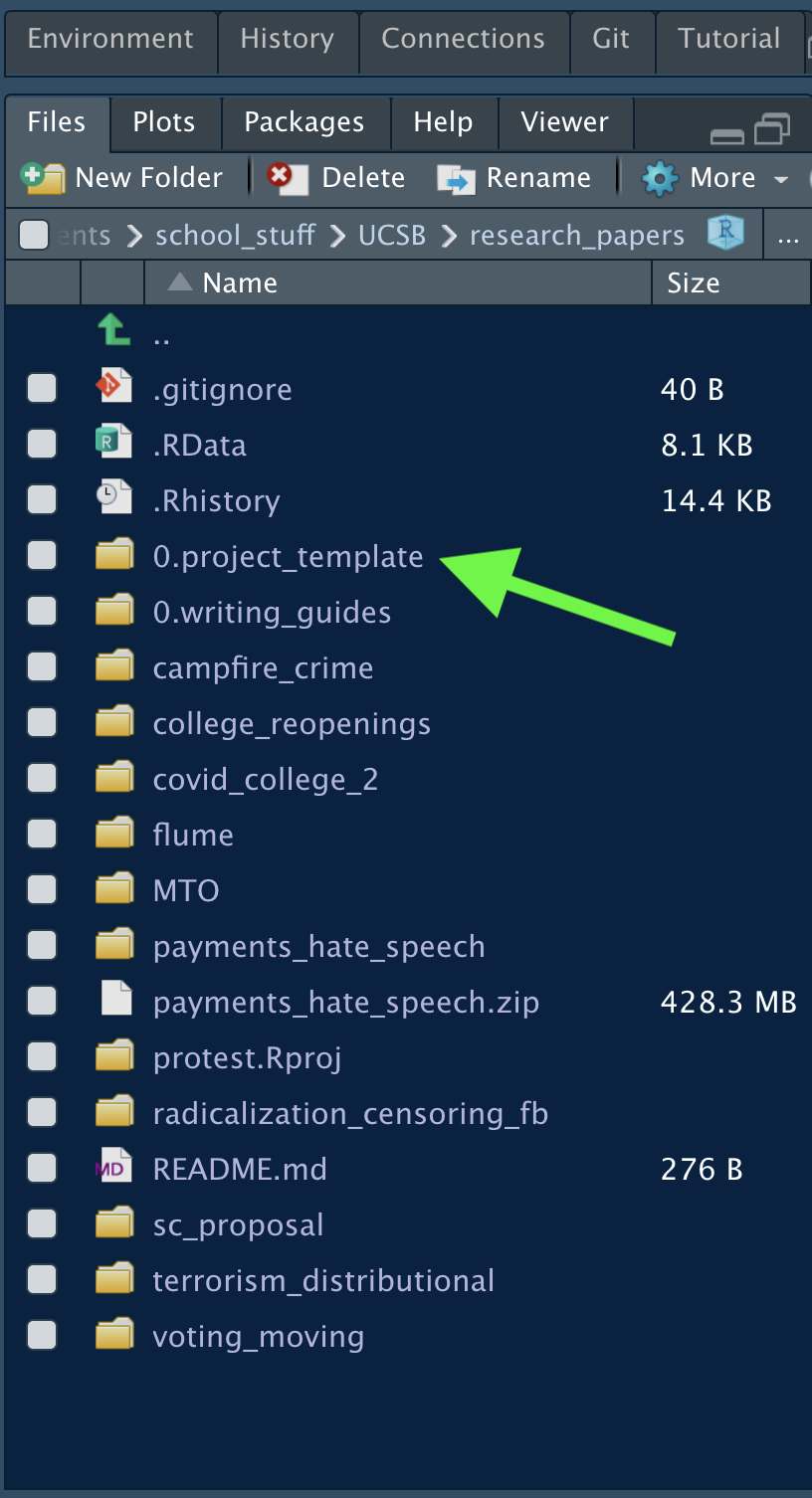
Figure 9.4: Having a Template
9.2 Rmarkdown
Rmarkdown is a native report compiler in R. It can be used to create many many things from .pdf, .docx, and .html files to interactive dashboards to websites. It’s impossible to cover everything in Rmarkdown in the span of a quarter, let alone a lecture. So we’ll focus on the basics.
Rmarkdown is an alternative to Latex compilers like Overleaf10. That means you can do all the same fancy math and formatting as if you were in Overleaf without ever leaving R. The benefits of Rmarkdown is the idea of code integration: you can directly run code in the document. This means you can pull data in and make a graph within your file automatically. If you update some data, the graph will update whenever you recompile. You can even have code in the middle of a sentence. You can write 2+2=4, but instead of writing 4, you can write `r ` with 2+2 following the r and it’ll solve it within line. If you’re discussing descriptive statistics in the body of your work, you no longer have to worry about copying and pasting the numbers wrong. It pulls directly from the data.
Today we’ll focus on the general setup of an Rmarkdown file and best practices we’ve learned for using Rmarkdown.
9.2.1 The Anatomy of an Rmarkdown File
You can create an Rmarkdown file just as you would an Rscript: File->New File-> R Markdown. After setting the name and type of output, you’ll be greeted with this file (or something quite similar):
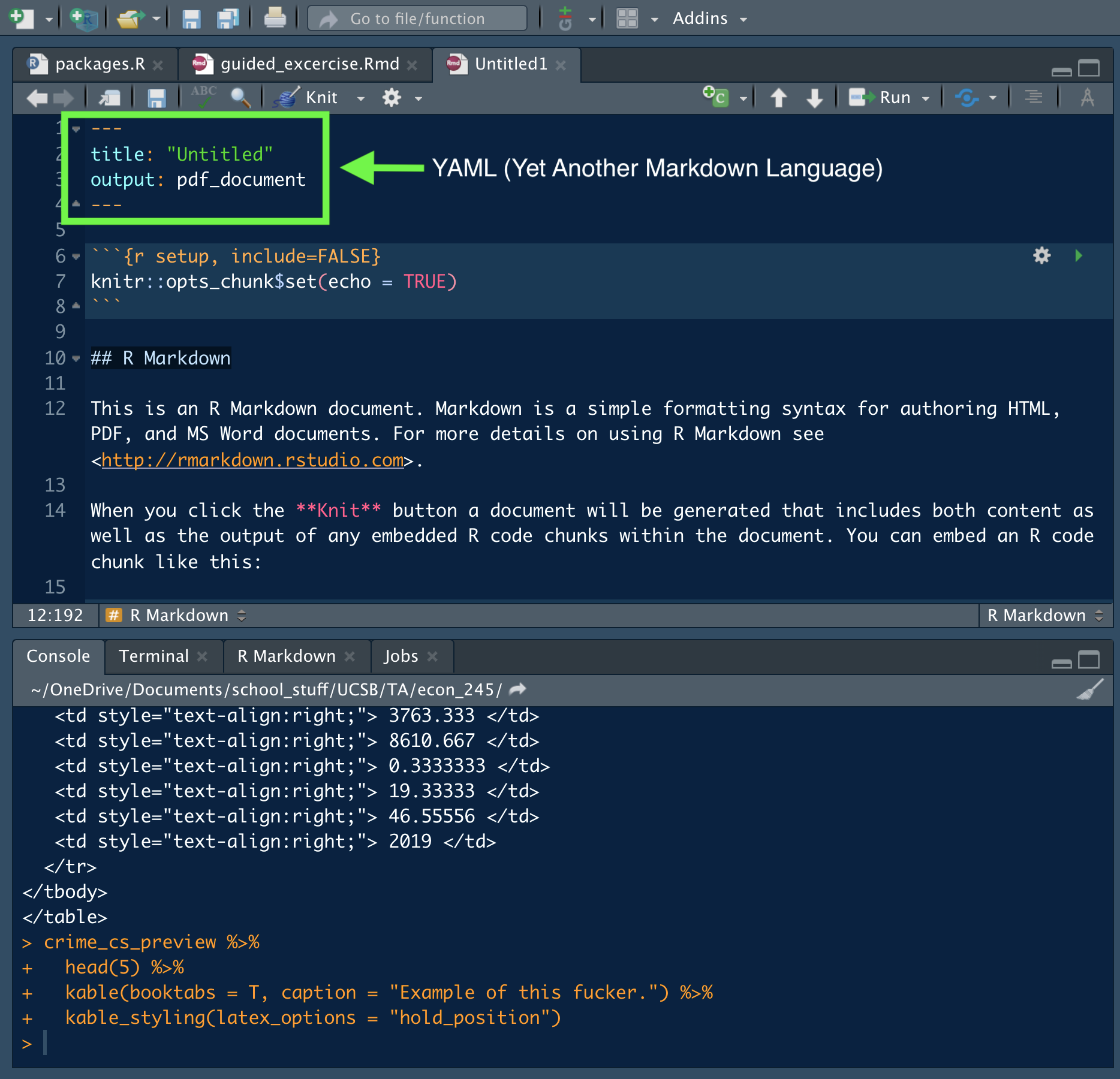
Figure 9.5: Basic Rmarkdown File
We’re going to focus on the top part, known as the YAML. This is where you set all the parameters for your document. Most YAMLs include things such as title, subtitle, author, and general paper preferences. An important note about the YAML is that indentation matters. Parameters end with a colon and parameters that are indented are read as sub-parameters. Below is an example of the YAML for a working paper as of 2021.
---
title: 'Indirect Financial Effects of Deplatforming'
subtitle: "Evidence from OwenBenjaminComedy"
author: Danny Klinenberg^[Ph.D. student at University of California, Santa Barbara;
  dklinenberg@ucsb.edu. All errors, omissions, and opinions are my own.]
date: 'Last Updated: 2023-06-10'
output:
  pdf_document:
    keep_tex: TRUE
    number_sections: yes
indent: yes
header-includes:
- \usepackage{amsfonts}
- \usepackage{amsthm}
- \usepackage{amsmath}
- \usepackage[english]{babel}
- \usepackage{bm}
- \usepackage{float}
- \usepackage[fontsize=12pt]{scrextend}
- \usepackage{graphicx}
- \usepackage{indentfirst}
- \usepackage[utf8]{inputenc}
- \usepackage{pdfpages}
- \usepackage[round,authoryear]{natbib}
- \usepackage{setspace}\doublespacing
- \usepackage{subfigure}
- \theoremstyle{definition}
- \newtheorem{definition}{Definition}[section]
- \newtheorem{assumption}{Assumption}
- \newtheorem{theorem}{Theorem}[section]
- \newtheorem{corollary}{Corollary}[theorem]
- \newtheorem{lemma}[theorem]{Lemma}
- \newtheorem*{remark}{Remark}
- \newcommand{\magenta}[1]{\textcolor{magenta}{#1}}
- \newcommand{\indep}{\perp \!\!\! \perp}
- \floatplacement{figure}{H}
- \bibliographystyle{plainnat}
- \pagenumbering{gobble}
- \usepackage{eso-pic,graphicx,transparent}
link-citations: yes
bibliography: references.bib
linkcolor: blue # magenta
abstract: \singlespacing I study things.
---
Rmarkdown also uses Latex packages. You add Latex packages under header-includes:. They should start with a dash space then slash just as you would do in any other Latex compiler.
Notice on line 41, there is a spot for a .bib file. You can add in-line citations by writing (_____?) and normal citations as (____?) where ____ is the reference code for the citation in your .bib file. Rmarkdown works with all normal bibliography software. Zotero is a great option because it’s free, can automatically create bibtex files, and is integrated with Rmarkdown and Microsoft Word.
There are many other options for the YAML and other ways to read in the parameters (such as a header.tex file) but we can stop here for now. The end of this discussion provides resources for in-depth questions on the matter.
Disclaimer: Setting up the YAML is not a one and done process most projects. It usually involves adding and removing Latex packages.
9.2.2 The Body of the Rmarkdown
The actual document is comprise of words, Latex, and code chunks. Below are some helpful tricks for writing in Rmarkdown:
A line beginning with one # signifies a section header.
A line beginning with two ## signifies a subsection header (and so on and so forth).
Dashes at the beginning of a line signify a bullet point.
One star around a word a phrase will italicize it. Two will bold it.
You can use all your favorite Latex commands in the body just as you would any other compiler.
The main benefit to Rmarkdown is the code chunk. You can create code chunk by pressing option+command+i on a Mac. You should see the following appear within your Rmarkdown file:
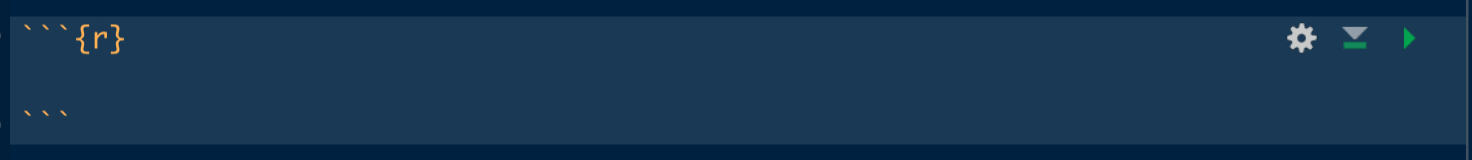
Figure 9.6: R code chunk
A code chunk operates just like it’s own little Rscript. Code chunks in an Rmarkdown file are all thought of as being part of the same Rscript, meaning they all use the same global environment. The top part of the code chunk, {r}, has a few options we’d like to highlight.
First, you can name your code chunks by adding a title after the r: ```{r example_code_chunk}. There can’t be any spaces in the code chunk. This is useful for quickly moving around your document.
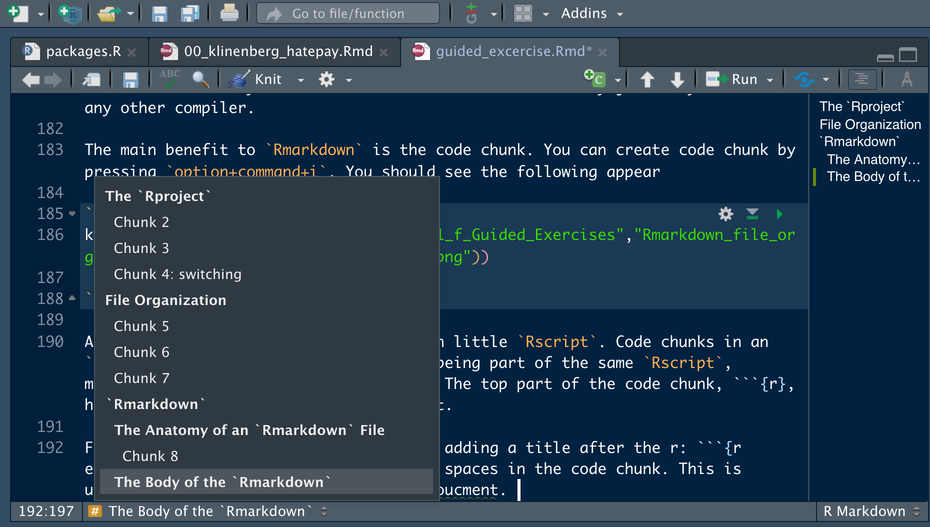
Figure 9.7: Quickly Moving
You can also choose what each code chunk does. To use these options, you write {r, option1=, option2=,…}. Below is a short list of the common settings you may be interested in:
echo: If you see the code in the document: echo=FALSE means you will not see the code.include: Whether or not the output is shown in the document.include=FALSEmeans the output will not be shown.eval: Whether or not the code is evaluated.
The code chunks will be most useful for integrating tables, images, and graphs. For example, the last image we saw was produced using the following code:
knitr::include_graphics(here::here("images", "organization","rmarkdown2.png"))Some useful options for figures and graphs are:
fig.cap: allows you to add a figure caption. You can make the figure reference-able by using label{}. For example, {r, fig.cap=“\\label{graph1} graph 1”} will allow you to reference graph 1 in the text by using \ref{graph1} Then the graph number in the text will always match the graph number in the title. If creating a graph natively using ggplot2/other graphing technique, you will still want to usefig.capso that the numbers automatically update correctly and you can reference the graphs in text.out.width: Allows you to change the size of the image or graph. examples would beout.width="50%".fig.align: If you want your figure to be centered, left justified, or right justified.
Finally, we can see that making tables becomes a painless process. The following code chunk creates a tibble to demonstrate how easy it is to make a table.
random_data<-tibble(y=rnorm(100,0,1),
                    x=y+4+rnorm(100,0,1)
                    )
Below, a simple regression is estimated. Using one line, the estimates are pushed to a publication-ready table as shown in Table \(\ref{table1}\).11
lm(y~x,data = random_data) %>%
modelsummary::modelsummary(title = "\\label{table1}A Publication-Quality Table")| (1) | |
|---|---|
| (Intercept) | −1.913 |
| (0.216) | |
| x | 0.483 |
| (0.049) | |
| Num.Obs. | 100 |
| R2 | 0.495 |
| R2 Adj. | 0.490 |
| AIC | 198.6 |
| BIC | 206.4 |
| Log.Lik. | −96.292 |
| F | 96.243 |
| RMSE | 0.63 |
With tables, you want to put the title in the table function. With graphs and images, you want to put the title in fig.cap at the top of the code chunk.
9.2.3 Childing
Research papers can be tens, if not hundreds, of pages long. No matter which compiler you choose, you will run into errors that will not let your paper compile. One way to limit this issue is to child parts of your paper into a main Rmarkdown file. Childing is to Rmarkdown as source is to R scripts. It allows us to tell Rmarkdown to go read in other .Rmd files. Figure \(\ref{files}\) shows a general setup for a research paper using Rmarkdown.
knitr::include_graphics(here::here("images", "organization","rmarkdown_3.png"))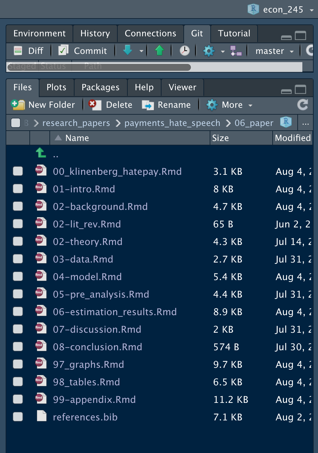
Figure 9.8: Rmarkdown Research Paper
File 00_klinenberg_hatepay.Rmd is the master file that brings all the other files in. This is where we put our YAML information and bring the other files in. Figure \(\ref{main_rmd}\) shows the beginning of the master .Rmd with the YAML collapsed form view.
knitr::include_graphics(here::here("images", "organization","rmarkdown4.png"))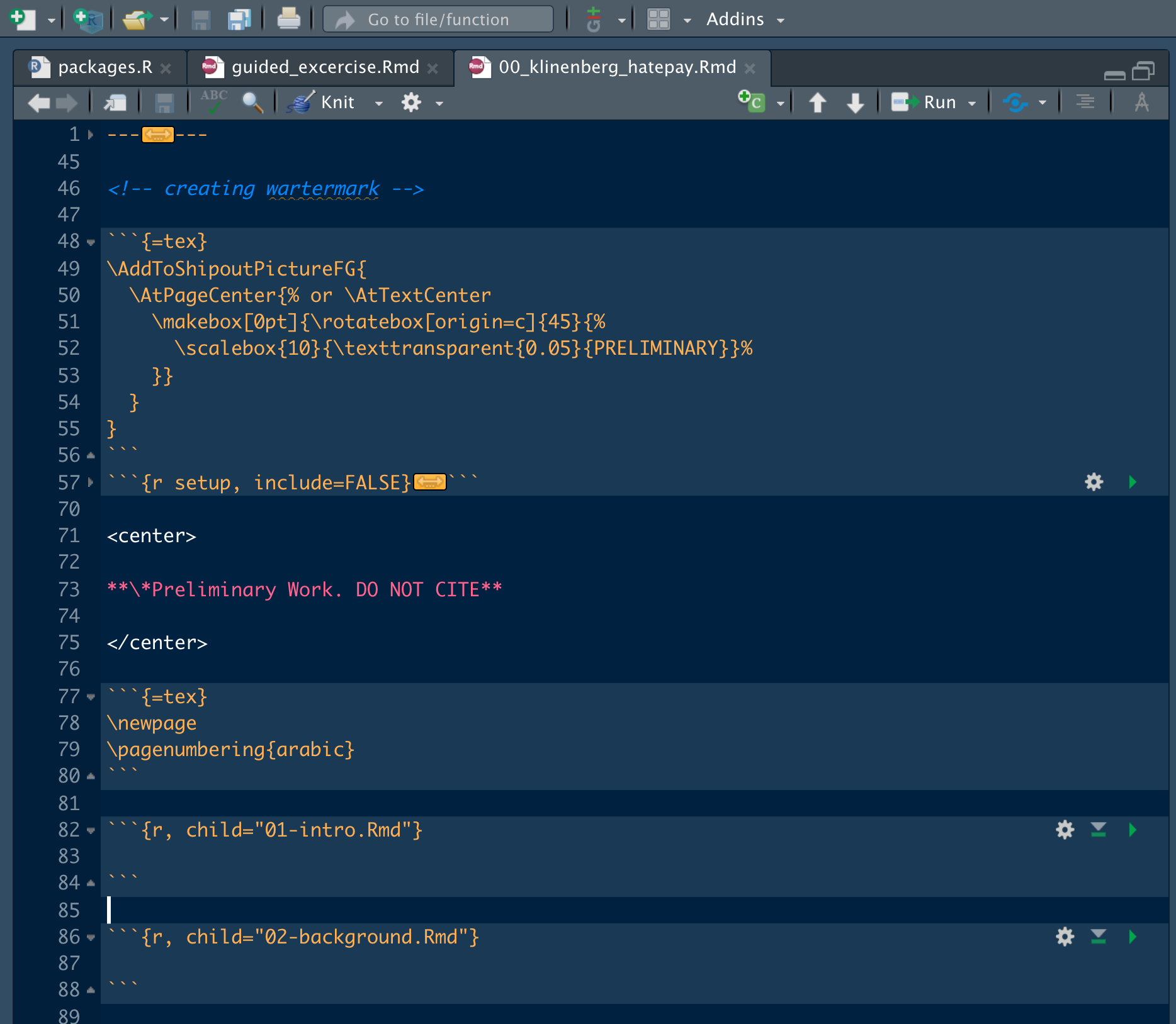
Figure 9.9: Example Master Rmarkdown File
Notice lines 82 and 86. The R header has the child option chosen and nothing else. This means that the R chunk will read the file as it’s execution. If you don’t have all the files next to each other, make sure to properly specify the file path.
Now, if your paper is not compiling, you do not have to go through the entire paper. You can individually load each .Rmd file and run it in isolation. Hence, you only need to debug 1-2 pages rather than 50.
9.2.4 Bibliographies
You can specify where the bibliography will go by writing the following lines in a Rmarkdown file:
# References {.unnumbered}

::: {#refs}
:::
You can also specify when the appendix begins (meaning you have different numbering) by writing:
\appendixRmarkdown works with all the Latex commands you already know. For example, I like to have the appendix of my papers restart page numbers at 1 and have my tables and graphs renumber starting with A1. To do that, I include the following Latex code below the YAML of my appendix.RMD file:
    \appendix
    \renewcommand{\thefigure}{A\arabic{figure}} \setcounter{figure}{0}
    \renewcommand{\thetable}{A\arabic{table}} \setcounter{table}{0}
    \renewcommand{\theequation}{A\arabic{table}} \setcounter{equation}{0}
    \setcounter{page}{1}
9.2.5 A Final Note on Rmarkdown: Visual Markdown Editor
A final note is the recent addition of the visual markdown editor. This is an html interface that blends the best of the Microsoft suite and Latex. You can access this by clicking the compass in the top right corner:
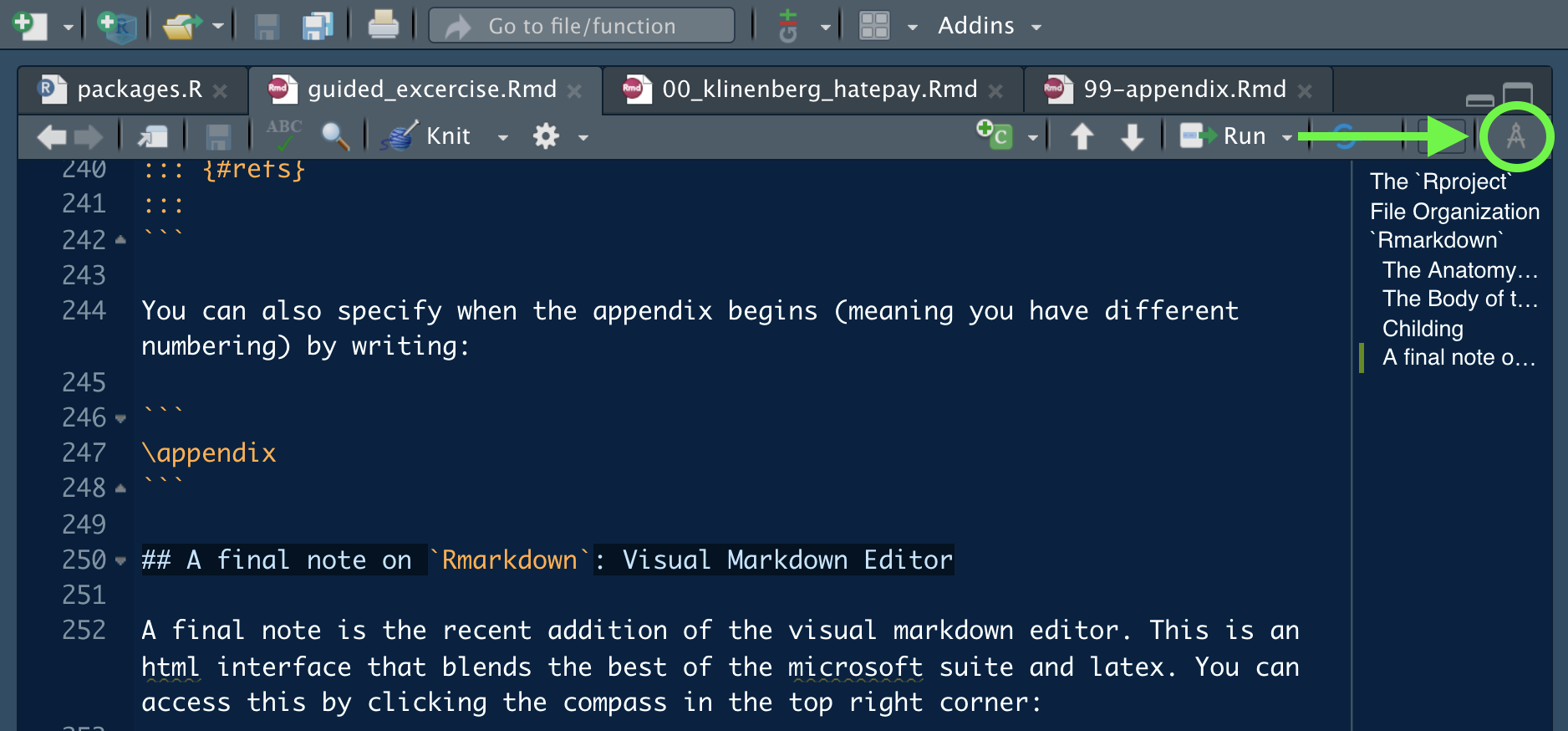
Figure 9.10: Enter the Editor
When you enter the visual markdown editor, you should notice a few things. First, headers look like headers. Second, we now have options at the top of the toolbar. These options include bolding, italicizing and underlining. We also have the option to use the GUI interface to make bullet points and add in citations (using @). The citation feature integrates with all major citation softwares (like Zotero) and automatically creates a .bib file in the same folder as your .RMD file.
There is much, much, more to learn about Rprojects, organization, and Rmarkdown. This served as an introduction to best practices, provided useful guides, and was an overview of what can be done. Here are some recommended additional readings:
If Hadley Wickam or Yihue Xie wrote it, then it’s worth reading.